Supervised learning
Classification
Bayesian Learners
Numerical, Categorical
Fast, Probabilities

One of my quirky videos from the “5 Minutes with Ingo” series. It explains the basic concepts of Naive Bayes in 5 minutes. And has unicorns.
Concept
Despite its simplicity, Naïve Bayes is a powerful machine learning technique. It only requires one single data scan for building the model. This is as fast as it can get. And for many problems, it shows excellent results. Learn more about this classifier below and make it part of your standard toolbox.
Let’s start with a small example. Somebody asks you to predict if a given day is a summer day or if this is a day in the middle of winter. Hence, the two classes of our classification problem are “summer” and “winter”. All this person is telling you about this day is that it is raining. You do not know anything else. What do you think? Is this rainy day a summer day or a winter day?
The answer obviously depends on where you are living. People from North America or Europe will often say: “It is probably a winter day since it rains much more in winter.”
This seems to be true. Below is the average amount of precipitation for Seattle, WA, USA – a town which is well known for having a lot of rain:
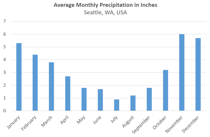
The average amount of rain per month in Seattle, WA, USA. Seattle is known for two things: lots of rain and lots of hospitals. Including made-up ones like the one from the TV show Grey’s Anatomy.
And this argument is exactly the basic idea of a Naïve Bayes classifier. It generally rains more in winter than in summer. If all I know is that the day in question is rainy, it is just more likely that this is a winter day. Case closed.
This thought leads to the concept of conditional probabilities and the Bayes rule. We will discuss the theory behind this a little bit later. For now, it is sufficient to know that we can use this rule to infer the probabilities for all possible classes based on the given observations.
The basic idea is easy to grasp from the image below. We can see that we have roughly the same amount of summer and winter days. Based on this alone, the probability that any given time would be winter day is about 50%:
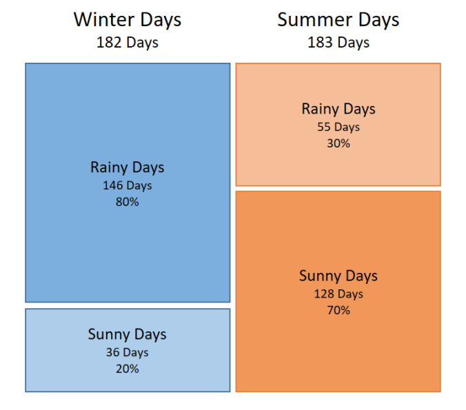
We have roughly the same amount of winter and summer days. So for any given day the probability to be a summer day is about 50%. But 80% of all days in winter are rainy and only 30% of days in summer. This knowledge reduces the probability for being a summer day.
But if you also factor in that the day in question is rainy, then this probability changes a bit. We will see later that we can calculate a likelihood of the day being a winter day if we know it is a rainy day. This likelihood is 80% * 50% = 40%. While the likelihood of being a summer day when it rains is only 30% * 50% = 15%. The likelihood that the day is in winter is much higher which leads us to the desired decision: it probably is a winter day!
Keep in mind that the outcome can also depend on a combination of events (“it rains and temperature is low”) instead of a single event (“it rains”). In machine learning, we represent such a combination of events as attributes or features of each observation. You could for example measure if it is raining or not, what the temperature is, and the wind speed. Those three factors, or events, would then become the attributes in your data set. And here is where the Naïve Bayes algorithm makes a somewhat naïve assumption (hence the name). The algorithm treats all attributes in the same way, i.e. it assumes that all attributes are equally important. And it also assumes that they are statistically independent of each other. This means that knowing the value of one attribute says nothing about the value of another. We can see already in our simple weather example that this assumption is never correct. A windy, rainy day usually also has a lower temperature.
But – and this is the surprising thing – although this naïve assumption is almost always incorrect, this machine learning scheme works very well in practice.
Theory
We will now translate the idea described above into an algorithm. We can use it to classify new observations based on the probabilities seen in past data. Let’s discuss a slightly more complex example which is still related to weather data. Below is a table with 14 observations (or “examples”). For each observation, we have some weather information, such as the outlook or the temperature. We also know the humidity and if the day was windy or not. This is the information we base our decisions on. We also have another column in the data which is our target, i.e. the attribute we want to predict. Let’s call this “play”, and this target attribute indicates if we are going on a round of golf or not.
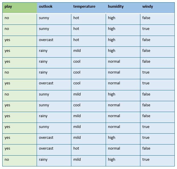
The Golf data set. We want to predict if somebody goes on a round of golf or not based on weather information like outlook or temperature. Not that true golfers would care. They always play.
Our Naïve Bayes algorithm is now very simple. First, you go through the data set once and count how often each combination of an attribute value (like “sunny”, “overcast”, or “rainy”) with each of the possible classes (here: “yes” or “no”) occurs. This leads to a much more compact representation of the information in the data set:
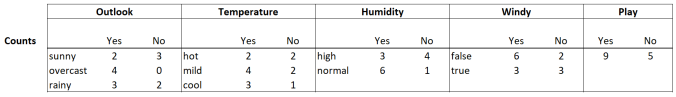
We can count all combinations of the attribute values with the possible values for the target “Play”. This can be done in a single data scan.
For example, you got 4 cases of days with a mild temperature at which you have been playing golf in the past. And 2 cases of mild days where you did not play. The beautiful thing is that you can generate all combination counts in the same data scan. This makes the algorithm very efficient.
The second step of the Naïve Bayes algorithm turns those counts into probabilities. We can simply divide each count by the number of observations in each class. We have 9 observations with Play = Yes and 5 cases with Play = No. Therefore, we divide the counts for the “Yes” combinations by 9 and the counts for combinations with “No” by 5:
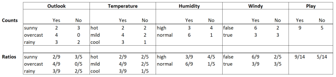
We turn the counts from above into ratios by dividing each count by the number of corresponding cases, i.e. 9 for “Yes” and 5 for “No”. We also calculate the overall ratios for “Yes” and “No” which are 9/14 and 5/14.
In the same step, we can also turn the counts for “Yes” and “No” into the correct probabilities. To do so, we divide them by the total number of observations in our data which is 14.
Those two simple steps are all you are doing for modeling in fact. The model can now be applied whenever you want to find out what the most likely outcome is for a new combination of weather events. This phase is also called “scoring”.
Let’s assume that we have a new day which is sunny and cool, but has a high humidity and is windy. We calculate the likelihood for playing golf on such a day by multiplying the ratios which correspond to the combination of those weather attributes with “yes”. The table below highlights those ratios:
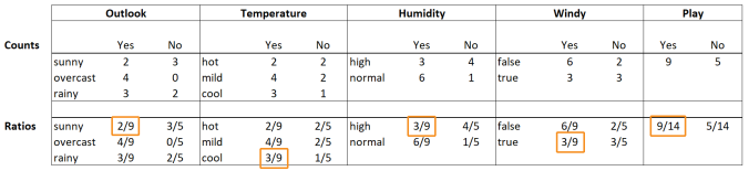
For a new prediction, we use the ratios of the weather condition at hand for each of the potential classes “Yes” and “No”. Above we can see the ratios in combination with “Yes”.
The likelihood for “yes” is then 2/9 * 3/9 * 3/9 * 3/9 * 9/14. The first four factors are the conditional probabilities that the specific weather events occur on a golfing day. The last probability, 9/14, is the overall probability to play golf independent of any weather information.
If you calculate the result for this formula you will end up with a likelihood of 0.0053.
We can now do the same calculation for our day (sunny, cool, high, true), but this time we assume that the day might be not a good day for golfing:
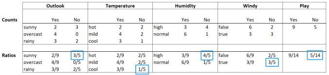
Finally, we can also calculate the likelihood for “No” by multiplying up the ratios of the weather conditions for the “No” case.
What is the likelihood for “no” in this case? We multiply the ratios which are 3/5 * 1/5 * 4/5 * 3/5 * 5/14 which results in 0.0206.
You can see that the total likelihood for “no” (0.0206) is much higher than the one for “yes” (0.0053). Therefore, our prediction for this day would be “no”. By the way, you can turn these likelihoods into true probabilities. Simply divide both values by the sum of them. The probability for “no” then is 0.0206 / (0.0206 + 0.0053) = 79.5% and the probability for “yes” is 0.0053 / (0.0053 + 0.0206) = 21.5%. Which confirms that we should not do a round of golf on such a day…
This is great. But how did we come up with the multiplication formula above? This where the Bayes Theorem comes into play.
This theorem states that

In our example, A means “yes, we play golf” and B means a specific weather condition like the one above. This is exactly the probability we are looking for. Is it likely that we play or not? We calculate this by multiplying the probability for the weather condition B given that we play (=P(B|A)) with the probability for playing (=P(A)). The latter one is very simple. This is just the ratio of yes-cases divided by the total number of observations, i.e. 5/14.
But what about P(B|A), i.e. the probability for a certain weather condition given that we play golf on such a day? This is exactly where the naïve assumption of attribute independence comes into play. If the attributes are independent of each other, we can calculate this probability by multiplying the elements:
![]()
where B1,…,Bm are the m attributes of our data set. And this is exactly the multiplication we have used above.
Finally, what happens to P(B) in the denominator of the Bayes theorem? In our example, this would be the likelihood of a certain weather condition independent of the question of playing golf. We do not know about this probability from our data above, but this is not a problem. Since we are only interested in the prediction “yes” or “no”, we can omit this probability. The reason is that the denominator would be the same for both cases. And therefore, it would not influence the ranking of the likelihoods. This is also the reason why we are only up with likelihoods above and not with true probabilities. To turn them into probabilities again we needed to divide the likelihoods by their sum.
Practical Usage
As pointed out above, Naïve Bayes should be another standard tool in your toolbox. It only requires a single data scan which makes it one of the fastest machine learning methods available. It often has a good accuracy even though the naïve assumption of attribute independence is often not fulfilled.
There is a downside though. The model is not easy to understand. You cannot see how the interaction of all attributes affects the outcome of the prediction.
Data Preparation
The algorithm is very robust and works on a variety of data types. We only have discussed categorical data above but it also works well on numerical data. Instead of counting, you calculate the mean values and standard deviations for the numerical values depending on the class. You can then use Gaussian distributions to estimate the probabilities for the values given each class. Some more sophisticated versions of the algorithm even allow to create more complex estimations for the distributions by using so-called kernel functions. But in both cases, the result will be a probability for the given value just like we got them for nominal attributes and their counts.
Alternatively, you can of course discretize your numerical column before you use Naïve Bayes.
Finally, most implementations of Naïve Bayes cannot deal with missing values. You need to take care of this before you build the model in such a case.
Parameters to Tune
One of the most beautiful things about Naïve Bayes is that it does not need the tuning of any parameters. If you have a more fancy version of the algorithm which uses kernel functions on numerical data, you might need to define the number of kernels used or similar parameters.
Memory Usage & Runtimes
We mentioned before that the algorithm only requires a single data scan to build the model. This makes it one of the fastest algorithms available.
Memory consumption is usually also quite moderate. The algorithm transforms the data into a table of counts. The size of this table depends on the number of classes you are predicting. It also depends on the number of attributes and how many different values each can take. While this can grow a bit, it usually is smaller than the original data table or not much bigger at least.
The runtime for scoring is also very fast. After all, you only look up the correct ratios for all attribute values and multiply them all. This does not cost a lot of time.
RapidMiner Processes
You can download RapidMiner here. Then you can download the process below to build this machine learning model yourself in RapidMiner.
- Train and apply a Naïve Bayes model: bayes_training_scoring
Please download the Zip-file and extract its content. The result will be an .rmp file which can be loaded into RapidMiner via “File” -> “Import Process…”.
