Basic Concepts of Feature Selection

Feature selection can greatly improve your machine learning models. In this series of blog posts, we will discuss all you need to know about feature selection.

  1. We start with explaining why feature selection is important – even in the age of deep learning. We then move on and establish that feature selection is actually a very hard problem to solve. We will cover different approaches which used today but have their own problems. This concludes the first blog post.
  2. We will then explain why evolutionary algorithms are one of the best solutions. We will discuss how they work and why they perform well even for large feature subsets.
  3. In the third post, we will improve the proposed technique. We will simultaneously improve the accuracy of models and reduce their complexity. This is the holy grail of feature selection. The proposed method should become your new standard technique.
  4. We will end with a discussion about feature selection for unsupervised learning. It turns out that you can use the multi-objective approach even in this case. Many consider feature selection for clustering to be an unsolved problem. But by using the proposed technique you can get better clustering results as well!

Ok, so let’s get started by defining the basics of feature selection first.

Why should we care about Feature Selection?

There is consensus that feature engineering often has bigger impact on the quality of a model than the model type or its parameters. And feature selection is a key part of feature engineering. Also, Kernel functions and hidden layers are performing implicit feature space transformations. So, is feature selection then still relevant in the age of SVMs and Deep Learning? The answer is: Yes, absolutely!

First, you can fool even the most complex model types. If there is enough noise overshadowing the true patterns, it will be hard to find them. The model starts to model the noise patterns of the unnecessary features in those cases. And that means, that it does not perform well at all. Or, even worse, it starts to overfit to those noise patterns and will fail on new data points. It turns out that it even easier to fall into this trap for high number of data dimensions. And no model type is better than others in this regard. Decision trees can fall into this trap as well as multi-layer neural networks. Removing noisy feature can help the model to focus on the relevant patterns instead.

But there are two more advantages of feature selection. If you reduce the number of features, models are generally trained much faster. And the resulting model often is simpler which makes it easier to understand. And more importantly, simpler models tend to be more robust. This means that they will perform better on new data points.

To summarize, you should always try to make the work easier for your model. Focus on the features which carry the signal over those which are noise. You can expect more accurate models and train them faster. Finally, they are easier to understand and are more robust. Sweet.

Why is this a hard problem?

Let’s begin with an example. We have a data set with 10 attributes (features, variables, columns…) and one label (target, class…). The label column is the one we want to predict. We trained a model on this data and evaluated it. The accuracy of the model built on the complete data was 62%. Is there any subset of those 10 attributes where a trained model would be more accurate than that? This is exactly the question feature selection tries to answer.

We can depict any attribute subset of 10 attributes as bit vectors, i.e. as a vector of 10 binary numbers 0 or 1. A 0 means that the specific attribute is not used while a 1 depicts an attribute which used for this subset. If we, for example, want to indicate that we use all 10 attributes, we would use the vector (1 1 1 1 1 1 1 1 1 1). Feature selection is the search for such a bit vector leading to a model with optimal accuracy. One possible approach for this would be to try out all the possible combinations. We could go through them one by one and evaluate how accurate a model would be using only those subsets. Let’s start with using only a single attribute then. The first bit vector looks like this:

picture1-1024x87As you can see, we only use the first attribute and a model only built on this subset has an accuracy of 68%. That is already better than what we got for all attributes which was 62%. But maybe we can improve even more? Let’s try using only the second attribute now:

picture2-1024x129
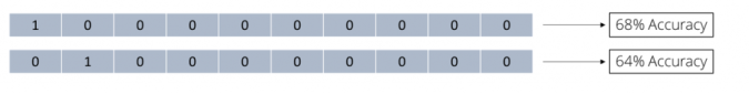
Still better than using all 10 attributes but not as good as only using the first. But let’s keep trying:

picture3-768x151
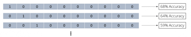
We keep going through all possible subsets of size 1 and collect all accuracy values. But why we should stop there? We should also try out subsets of 2 attributes now:

picture4-1024x306
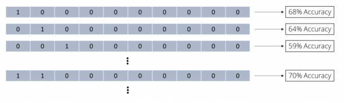
Using the first two attributes immediately looked promising with 70% accuracy. We keep going through all possible subsets of all possible sizes. We collect all accuracy values of those subsets until we tried all possible combinations:

picture5-1024x351
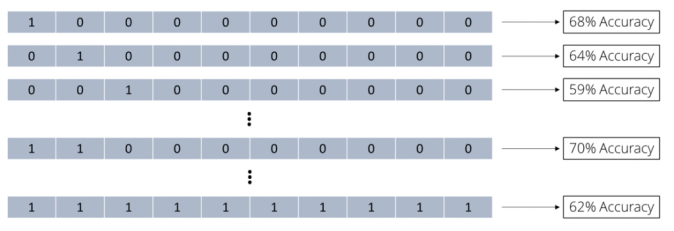
We now have the full picture and can use the best subset out of all these combinations. Because we tried all combinations, we also call this a brute force approach.

How many combinations did we try for our data set consisting of 10 attributes? We have two options for each attribute: we can decide to either use it or not. And we can make this decision for all 10 attributes which results in 2 x 2 x 2 x … = 210 or 1024 different outcomes. One of those combinations does not make any sense though, namely the one which does not use any features at all. So, this means that we only would try 210 – 1 = 1023 subsets. Anyway, even for a small data set with only 10 attributes this is already a lot of attribute subsets we need to try. Also keep in mind that we perform a model validation for every single one of those combinations. If we used a 10-fold cross-validation, we now trained 10230 models already. That is a lot. But it is still doable for fast model types on fast machines.

But what about more realistic data sets? This is where the trouble begins. If we have 100 instead of only 10 attributes in our data set, we already have 2100 – 1 combinations. This brings the total number of combinations already to 1,267,650,600,228,229,401,496,703,205,375. Even the biggest computers can no longer do this. This rules out such a brute force approach for any data set consisting of more than just a handful features.

Heuristics to the Rescue!

Going through all possible attribute subsets is not a feasible approach then. But what can we do instead? We could try to focus only on such combinations which are more likely to lead to more accurate models. We try to prune the search space and ignore feature sets which are not likely to produce good models. However, there is of course no guarantee that you will find the optimal solution any longer. If you ignore complete areas of your solution space, it might be that you also skip the optimal solution. But at least such heuristics are much faster than the brute force approach. And often you will end up with a good and sometimes even with the optimal solution in a much faster time.

There are two widely used approaches for feature selection heuristics in machine learning. We call them forward selection and backward elimination. The heuristic behind forward selection is very simple. you first try out all subsets with only one attribute and keep the best solution. But instead of trying all possible subsets with two features next, you only try specific 2-subsets. You only try those 2-subsets which contain the best attribute from the previous round. If you do not improve, you stop and deliver the best result from before, i.e. the single attribute. But if you have improved the accuracy, you keep trying by keeping the best attributes so far and try to add one more. You keep doing this until you no longer improve.

What does this mean for the runtime for our example with 10 attributes from above? We start with the 10 subsets of only one attribute which is 10 model evaluations. We then keep the best performing attribute and try the 9 possible combinations with the other attributes. This is another 9 model evaluations then. We stop if there is no improvement or keep the best 2-subset if we got a better accuracy. We now try the 8 possible 3-subsets and so on. So, instead of going brute force through all 1023 possible subsets, we only go through 10 + 9 + … + 1 = 55 subsets. And we often will stop much earlier as soon as there is no further improvement. We will see below that this is often the case. This is an impressive reduction in runtime. And the difference becomes even more obvious for the case with 100 attributes. Here we will only try at most 5,050 combinations instead of the 1,267,650,600,228,229,401,496,703,205,375 possible ones.

Things are similar with backward elimination, we just turn the direction around. We begin with the subset consisting of all attributes first. Then, we try to leave out one single attribute at a time. If we improved, we keep going. But we still leave out the attribute which led to the biggest improvement in accuracy. We then go through all possible combinations by leaving out one more attribute. This is in addition to the best ones we left already out before. We continue doing this until we no longer improve. Again, for 10 attributes this means that we will have at most 1 + 10 + 9 + 8 + … + 2 = 55 combinations we need to evaluate.

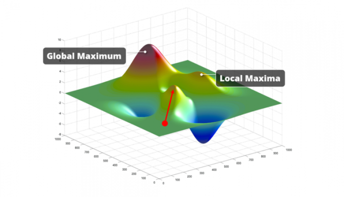
Are we done then? It looks like we found some heuristics which work much faster than the brute force approach. And in certain cases, these approaches will deliver a very good attribute subset. The problem is that in most cases, they unfortunately will not. For most data sets, the model accuracy values form a so-called multi-modal fitness landscape. This means that besides one global optimum there are several local optima as well. Both methods will start somewhere on this fitness landscape and will move from there. In the image below, we marked such a starting point with a red dot. From there, they will continue to add (or remove) attributes if the fitness improves. They will always climb up the nearest hill in the multi-modal fitness landscape. And if this hill is a local optimum they will get stuck in there since there is no further climbing possible. Hence, those algorithms do not even bother with looking out for higher hills. They take whatever they can easily get. Which is exactly why we call those algorithms “greedy” by the way. And when they stop improving, there is only a very small likelihood that they made it on top of the highest hill. It is much more likely that they missed the global optimum we are looking for. Which means that the delivered feature subset is often a sub-optimal result.

picture6-768x441

Slow vs. Bad. Anything better out there?

This is not good then, is it? We have one technique which would deliver the optimal result, but is computationally not feasible. This is the brute force approach. But as we have seen, we cannot use it at all on realistic data sets. And we have two heuristics, forward selection and backward elimination, which deliver results much quicker. But unfortunately, they will run into the first local optimum they find. And that means that they most likely will not deliver the optimal result. Don’t give up though – in the next post we will discuss another heuristic which is still feasible even for larger data sets. And it often delivers much better results than forward selection and backward elimination. This heuristic is making use of evolutionary algorithms which will be the topic of the next post.

Naïve Bayes – Not so naïve after all!

Family:
Supervised learning
Modeling types:
Classification
Group:
Bayesian Learners
Input data:
Numerical, Categorical
Tags:
Fast, Probabilities
5MwI_bayes

One of my quirky videos from the “5 Minutes with Ingo” series. It explains the basic concepts of Naive Bayes in 5 minutes. And has unicorns.

Concept

Despite its simplicity, Naïve Bayes is a powerful machine learning technique.  It only requires one single data scan for building the model.  This is as fast as it can get.  And for many problems, it shows excellent results.  Learn more about this classifier below and make it part of your standard toolbox.

Let’s start with a small example.  Somebody asks you to predict if a given day is a summer day or if this is a day in the middle of winter.  Hence, the two classes of our classification problem are “summer” and “winter”.  All this person is telling you about this day is that it is raining.  You do not know anything else.  What do you think?  Is this rainy day a summer day or a winter day?

The answer obviously depends on where you are living.  People from North America or Europe will often say: “It is probably a winter day since it rains much more in winter.”

This seems to be true.  Below is the average amount of precipitation for Seattle, WA, USA – a town which is well known for having a lot of rain:

nb_seattle_precipitation

The average amount of rain per month in Seattle, WA, USA.  Seattle is known for two things: lots of rain and lots of hospitals.  Including made-up ones like the one from the TV show Grey’s Anatomy.

And this argument is exactly the basic idea of a Naïve Bayes classifier.  It generally rains more in winter than in summer.  If all I know is that the day in question is rainy, it is just more likely that this is a winter day.  Case closed.

This thought leads to the concept of conditional probabilities and the Bayes rule.  We will discuss the theory behind this a little bit later.  For now, it is sufficient to know that we can use this rule to infer the probabilities for all possible classes based on the given observations.

The basic idea is easy to grasp from the image below.  We can see that we have roughly the same amount of summer and winter days.  Based on this alone, the probability that any given time would be winter day is about 50%:

nb_rainy_day

We have roughly the same amount of winter and summer days.  So for any given day the probability to be a summer day is about 50%.  But 80% of all days in winter are rainy and only 30% of days in summer.  This knowledge reduces the probability for being a summer day.

But if you also factor in that the day in question is rainy, then this probability changes a bit.  We will see later that we can calculate a likelihood of the day being a winter day if we know it is a rainy day.  This likelihood is 80% * 50% = 40%.  While the likelihood of being a summer day when it rains is only 30% * 50% = 15%.  The likelihood that the day is in winter is much higher which leads us to the desired decision: it probably is a winter day!

Keep in mind that the outcome can also depend on a combination of events (“it rains and temperature is low”) instead of a single event (“it rains”).  In machine learning, we represent such a combination of events as attributes or features of each observation.  You could for example measure if it is raining or not, what the temperature is, and the wind speed.  Those three factors, or events, would then become the attributes in your data set.  And here is where the Naïve Bayes algorithm makes a somewhat naïve assumption (hence the name).  The algorithm treats all attributes in the same way, i.e. it assumes that all attributes are equally important.  And it also assumes that they are statistically independent of each other.  This means that knowing the value of one attribute says nothing about the value of another.  We can see already in our simple weather example that this assumption is never correct.  A windy, rainy day usually also has a lower temperature.

But – and this is the surprising thing – although this naïve assumption is almost always incorrect, this machine learning scheme works very well in practice.

Theory

We will now translate the idea described above into an algorithm. We can use it to classify new observations based on the probabilities seen in past data.  Let’s discuss a slightly more complex example which is still related to weather data.  Below is a table with 14 observations (or “examples”).  For each observation, we have some weather information, such as the outlook or the temperature.  We also know the humidity and if the day was windy or not.  This is the information we base our decisions on.  We also have another column in the data which is our target, i.e. the attribute we want to predict.  Let’s call this “play”, and this target attribute indicates if we are going on a round of golf or not.

nb_golf_data

The Golf data set.  We want to predict if somebody goes on a round of golf or not based on weather information like outlook or temperature.  Not that true golfers would care.  They always play.

Our Naïve Bayes algorithm is now very simple.  First, you go through the data set once and count how often each combination of an attribute value (like “sunny”, “overcast”, or “rainy”) with each of the possible classes (here: “yes” or “no”) occurs. This leads to a much more compact representation of the information in the data set:

nb_data_counts

We can count all combinations of the attribute values with the possible values for the target “Play”.  This can be done in a single data scan.

For example, you got 4 cases of days with a mild temperature at which you have been playing golf in the past.  And 2 cases of mild days where you did not play.  The beautiful thing is that you can generate all combination counts in the same data scan.  This makes the algorithm very efficient.

The second step of the Naïve Bayes algorithm turns those counts into probabilities.  We can simply divide each count by the number of observations in each class.  We have 9 observations with Play = Yes and 5 cases with Play = No.  Therefore, we divide the counts for the “Yes” combinations by 9 and the counts for combinations with “No” by 5:

nb_data_ratios

We turn the counts from above into ratios by dividing each count by the number of corresponding cases, i.e. 9 for “Yes” and 5 for “No”.  We also calculate the overall ratios for “Yes” and “No” which are 9/14 and 5/14.

In the same step, we can also turn the counts for “Yes” and “No” into the correct probabilities.  To do so, we divide them by the total number of observations in our data which is 14.

Those two simple steps are all you are doing for modeling in fact.  The model can now be applied whenever you want to find out what the most likely outcome is for a new combination of weather events.  This phase is also called “scoring”.

Let’s assume that we have a new day which is sunny and cool, but has a high humidity and is windy.  We calculate the likelihood for playing golf on such a day by multiplying the ratios which correspond to the combination of those weather attributes with “yes”.  The table below highlights those ratios:

nb_data_ratios_likelihood_yes

For a new prediction, we use the ratios of the weather condition at hand for each of the potential classes “Yes” and “No”.  Above we can see the ratios in combination with “Yes”.

The likelihood for “yes” is then 2/9 * 3/9 * 3/9 * 3/9 * 9/14.  The first four factors are the conditional probabilities that the specific weather events occur on a golfing day.  The last probability, 9/14, is the overall probability to play golf independent of any weather information.

If you calculate the result for this formula you will end up with a likelihood of 0.0053.
We can now do the same calculation for our day (sunny, cool, high, true), but this time we assume that the day might be not a good day for golfing:

nb_data_ratios_likelihood_no

Finally, we can also calculate the likelihood for “No” by multiplying up the ratios of the weather conditions for the “No” case.

What is the likelihood for “no” in this case?  We multiply the ratios which are 3/5 * 1/5 * 4/5 * 3/5 * 5/14 which results in 0.0206.

You can see that the total likelihood for “no” (0.0206) is much higher than the one for “yes” (0.0053).  Therefore, our prediction for this day would be “no”.  By the way, you can turn these likelihoods into true probabilities.  Simply divide both values by the sum of them.  The probability for “no” then is 0.0206 / (0.0206 + 0.0053) = 79.5% and the probability for “yes” is 0.0053 / (0.0053 + 0.0206) = 21.5%.  Which confirms that we should not do a round of golf on such a day…

This is great.  But how did we come up with the multiplication formula above?  This where the Bayes Theorem comes into play.

This theorem states that

nb_formula_bayes.png

In our example, A means “yes, we play golf” and B means a specific weather condition like the one above.  This is exactly the probability we are looking for.  Is it likely that we play or not?  We calculate this by multiplying the probability for the weather condition B given that we play (=P(B|A)) with the probability for playing (=P(A)). The latter one is very simple. This is just the ratio of yes-cases divided by the total number of observations, i.e. 5/14.

But what about P(B|A), i.e. the probability for a certain weather condition given that we play golf on such a day? This is exactly where the naïve assumption of attribute independence comes into play. If the attributes are independent of each other, we can calculate this probability by multiplying the elements:

nb_formula_p_b_a.png

where B1,…,Bm are the m attributes of our data set.  And this is exactly the multiplication we have used above.

Finally, what happens to P(B) in the denominator of the Bayes theorem?  In our example, this would be the likelihood of a certain weather condition independent of the question of playing golf.  We do not know about this probability from our data above, but this is not a problem.  Since we are only interested in the prediction “yes” or “no”, we can omit this probability.  The reason is that the denominator would be the same for both cases.  And therefore, it would not influence the ranking of the likelihoods.  This is also the reason why we are only up with likelihoods above and not with true probabilities.  To turn them into probabilities again we needed to divide the likelihoods by their sum.

Practical Usage

As pointed out above, Naïve Bayes should be another standard tool in your toolbox.  It only requires a single data scan which makes it one of the fastest machine learning methods available.  It often has a good accuracy even though the naïve assumption of attribute independence is often not fulfilled.

There is a downside though.  The model is not easy to understand.  You cannot see how the interaction of all attributes affects the outcome of the prediction.

Data Preparation

The algorithm is very robust and works on a variety of data types.  We only have discussed categorical data above but it also works well on numerical data.  Instead of counting, you calculate the mean values and standard deviations for the numerical values depending on the class.  You can then use Gaussian distributions to estimate the probabilities for the values given each class.  Some more sophisticated versions of the algorithm even allow to create more complex estimations for the distributions by using so-called kernel functions.  But in both cases, the result will be a probability for the given value just like we got them for nominal attributes and their counts.

Alternatively, you can of course discretize your numerical column before you use Naïve Bayes.

Finally, most implementations of Naïve Bayes cannot deal with missing values.  You need to take care of this before you build the model in such a case.

Parameters to Tune

One of the most beautiful things about Naïve Bayes is that it does not need the tuning of any parameters.  If you have a more fancy version of the algorithm which uses kernel functions on numerical data, you might need to define the number of kernels used or similar parameters.

Memory Usage & Runtimes

We mentioned before that the algorithm only requires a single data scan to build the model.  This makes it one of the fastest algorithms available.

Memory consumption is usually also quite moderate.  The algorithm transforms the data into a table of counts.  The size of this table depends on the number of classes you are predicting.  It also depends on the number of attributes and how many different values each can take.  While this can grow a bit, it usually is smaller than the original data table or not much bigger at least.

The runtime for scoring is also very fast.  After all, you only look up the correct ratios for all attribute values and multiply them all.  This does not cost a lot of time.

RapidMiner Processes

You can download RapidMiner here.  Then you can download the process below to build this machine learning model yourself in RapidMiner.

Please download the Zip-file and extract its content.  The result will be an .rmp file which can be loaded into RapidMiner via “File” -> “Import Process…”.

What Artificial Intelligence and Machine Learning can do – and what not

I have written on Artificial Intelligence (AI) before.  Back then I focused on the technology side of it: what is part of an AI system and what isn’t.  But there is another question which might be even more important.  What are we DOING with AI?

Part of my job is to help investors with their due diligence.  I discuss companies with them in which they might want to invest. Here is a quick observation:  By now, every company pitch is full with stuff about how they are using AI to solve a given business problem.

Part of me loves this since some of those companies are on something and should get the chance.  But I also have a built-in “bullshit-meter”.  So, another part of me wants to cringe every time I listen to a founder making stuff up about how AI will help him.  I listened to many founders who do not know a lot about AI, but they sense that they can get millions of dollars of funding.  Just by adding those fluffy keywords to their pitch.  The bad news is that it sooner or later actually works.  Who am I to blame them?

I have seen situations where AI or at least machine learning (ML) has an incredible impact.  But I also have seen situations where this is not the case.  What was the difference?

In most of the cases where organizations fail with AI or ML, they used those techniques in the wrong context.  ML models are not very helpful if you have only one big decision you need to make.  Analytics still can help you in such cases by giving you easier access to the data you need to make this decision.  Or by presenting this data in a consumable fashion.  But at the end of the day, those single big decisions are often very strategic.  Building a machine learning model or an AI to help you making this decision is not worth doing it.  And often they also do not yield better results than just making the decision on your own.

Here is where ML and AI can help. Machine Learning and Artificial Intelligence deliver most value whenever you need to make lots of similar decisions quickly. Good examples for this are:

  • Defining the price of a product in markets with rapidly changing demands,
  • Making offers for cross-selling in an E-Commerce platform,
  • Approving a credit or not,
  • Detecting customers with a high risk for churn,
  • Stopping fraudulent transactions,
  • …among others.

You can see that a human being who would have access to all relevant data could make those decisions in a matter of seconds or minutes.  Only that they can’t without AI or ML, since they would need to make this type of decision millions of times, every day.  Like sifting through your customer base of 50 million clients every day to identify those with a high churn risk.  Impossible for any human being.  But no problem at all for an ML model.

So, the biggest value of artificial intelligence and machine learning is not to support us with those big strategic decisions.  Machine learning delivers most value when we operationalize models and automate millions of decisions.

The image below shows this spectrum of decisions and the times humans need to make those.  The blue boxes are situations where analytics can help, but it is not providing its full value. The orange boxes are situations where AI and ML show real value. And the interesting observation is: the more decisions you can automate, the higher this value will be (upper right end of this spectrum).

automating_decisions_with_ML_and_AI

One of the shortest descriptions of this phenomenon comes from Andrew Ng, who is a well-known researcher in the field of AI.  Andrew described what AI can do as follows:

“If a typical person can do a mental task with less than one second of thought, we can probably automate it using AI either now or in the near future.”

I agree with him on this characterization. And I like that he puts the emphasis on automation and operationalization of those models – because this is where the biggest value is. The only thing I disagree with is the time unit he chose. It is safe to go already with a minute instead of a second.

K-Nearest Neighbors – the Laziest Machine Learning Technique

Family:
Supervised learning
Modeling types:
Classification, Regression
Group:
Lazy Learners / Instance-based Learners
Input data:
Numerical, Categorical
Tags:
Fast, Local, Global
5MwI_knn

One of my quirky videos from the “5 Minutes with Ingo” series. It explains the basic concepts of k-Nearest Neighbors N in 5 minutes. And has unicorns.

Concept

k-Nearest Neighbors is one of the simplest machine learning algorithms.  As for many others, human reasoning was the inspiration for this one as well.  Whenever something significant happened in your life, you will memorize this experience.  You will later use this experience as a guideline about what you expect to happen next.

Consider you see somebody dropping a glass. While the glass falls, you already make the prediction that the glass will break when it hits the ground. But how can you do this? You never have seen THIS glass breaking before, right?

No, indeed not. But you have seen similar glasses or in general similar items dropping to the floor before.  And while the situation might not be exactly the same, you still know that a glass dropping from about 5 feet on a concrete floor usually breaks.  This gives you a pretty high level of confidence to expect breakage whenever you see a glass fall from that height on a hard floor.

But what about dropping a glass from a foot height onto a soft carpet?  Did you experience breaking glasses in such situations as well?  No, you did not.  We can see that the height matters, so does the hardness of the ground.

This way of reasoning is what a k-Nearest Neighbors algorithm is doing as well.  Whenever a new situation occurs, it scans through all past experiences and looks up the k closest experiences.  Those experiences (or: data points) are what we call the k nearest neighbors.

If you have a classification task, for example you want to predict if the glass breaks or not, you take the majority vote of all k neighbors.  If k=5 and in 3 or more of your most similar experiences the glass broke, you go with the prediction “yes, it will break”.

Let’s now assume that you want to predict the number of pieces a glass will break into.  In this case, we want to predict a number which we call “regression”.  Now you take the average value of your k neighbors’ numbers of glass pieces as a prediction or score.  If k=5 and the numbers of pieces are 1 (did not break), 4, 8, 2, and 10 you will end up with the prediction of 5.

knn_concept

We have blue and orange data points.  For a new data point (green), we can determine the most likely class by looking up the classes of the nearest neighbors.  Here, the decision would be “blue”, because that is the majority of the neighbors.

Why is this algorithm called “lazy”?  Because it does no training at all when you supply the training data.  At training time, all it is doing is storing the complete data set but it does not do any calculations at this point.  Neither does it try to derive a more compact model from the data which it could use for scoring.   Therefore, we call this algorithm lazy.

Theory

We have seen that this algorithm is lazy and during training time all it is doing is to store all the data it gets.  All the computation happens during scoring, i.e. when we apply the model on unseen data points.  We need to determine which k data points out of our training set are closest to the data point we want to get a prediction for.

Let’s say that our data points look like the following:

data_set_math

We have a table of n rows and m+1 columns where the first m columns are the attributes we use to predict the remaining label column (also known as “target”).  For now, let’s also assume that all attribute values x are numerical while the label values for y are categorical, i.e. we have a classification problem.

We can now define a distance function which calculates the distance between data points.  Especially, it should find the closest data points from our training data for any new point.  The Euclidean distance often is a good choice for such a distance function if the data is numerical.  If our new data point has attribute values s1 to sm, we can calculate the distance d(s, xj) between point s to any data point xj by

euclidean_distance_math

The k data points with the closest value for this distance become our k neighbors.  For a classification task, we now use the most frequent of all values y from our k neighbors.  For regression tasks, where y is numerical, we use the average of all values y from our k neighbors.

But what if our attributes are not numerical or consist of numerical and categorical attributes?  Then you can use any other distance measure which can handle this type of data.  This article discusses some frequent choices.

By the way, K-Nearest Neighbors models with k=1 are the reason why calculating training errors are completely pointless.  Can you see why?

Practical Usage

K-Nearest Neighbors, or short: K-NN, should be a standard tool in your toolbox.  It is fast, easy to understand even for non-experts, and it is easy to tune it to different kind of predictive problems.  But there are some things to consider which we will discuss in the following.

Data Preparation

We have seen that the key part of the algorithm is the definition of a distance measure.  A frequent choice is the Euclidean distance. This distance measure treats all data columns in the same way though. It subtracts the values for each dimension before it sums up the squares of those distances. And that means that columns with a wider data range have a larger influence on the distance than columns with a smaller data range.

So, you should normalize the data set so that all columns are roughly on the same scale. There are two common ways of normalization. First, you could bring all values of a column into a range between 0 and 1. Or you could change the values of each column so that the column has a mean 0 with a standard deviation of 1 afterwards. We call this type of normalization z-transformation or standard score.

Tip: Whenever you know that the machine learning algorithm is making use of a distance measure, you should normalize the data. Another famous example would be k-Means clustering.

Parameters to Tune

The most important parameter you need to tune is k, the number of neighbors used to make the class decision.  The minimum value is 1 in which case you only look at the closest neighbor for each prediction to make your decision.  In theory, you could use a value for k which is as large as your total training set.  This would make no sense though, since in this case you would always predict the majority class of the complete training set.

Here is a good way to interpret the meaning behind k. Small numbers indicate “local” models, which can be non-linear and the decision boundary between the classes wiggle a lot. If the number grows, the wiggling gets less until you almost end up with a linear decision boundary.

knn_impact_of_k

We see a data set in two dimensions on the left.  In general the top right is red and the bottom left is the blue class.  But there are also some local groups inside of both areas.  Small values for k lead to more wiggly decision boundaries.  For larger values the decision boundary becomes smoother, almost linear in this case.

Good values for k depend on the data you have and if the problem is non-linear or not.  You should try a couple of values between 1 and about 10% of the size of the training data set size.  Then you will see if there is a promising area worth the further optimization of k.

The second parameter you might want to consider is the type of distance function you are using.  For numerical values, Euclidean distance is a good choice.  You might want to try Manhattan distance which is sometimes used as well.  For text analytics, cosine distance can be another good alternative worth trying.

Memory Usage & Runtimes

Please note that all this algorithm is doing is storing the complete training data.  So, the memory needs grow linearly with the number of data points you provide for training.  Smarter implementations of this algorithm might choose to store the data in a more compact fashion.  But in a worst-case scenario you still end up with a lot of memory usage.

For training, the runtime is as good as it gets.  The algorithm is doing no calculations at all besides storing the data which is fast.

The runtime for scoring though can be large though which is unusual in the world of machine learning.  All calculations happen during model application.  Hence, the scoring runtime scales linearly with the number of data columns m and the number of training points n.  So, if you need to score fast and the number of training data points is large, then k-Nearest Neighbors is not a good choice.

RapidMiner Processes

You can download RapidMiner here.  Then you can download the processes below to build this machine learning model yourself in RapidMiner.

Please download the Zip-file and extract its content.  The result will be an .rmp file which can be loaded into RapidMiner via “File” -> “Import Process…”.

So, what is Data Science then?

I just finished a post on explaining the relationship between Artificial Intelligence, Machine Learning, and Deep Learning.  And somebody immediately pointed out: But what about Data Science? How does Data Science relate to all this?

Good question.  That’s what I am going to write about today then.

In case you do not want to read the whole post from yesterday (shame on you!), here is a quick summary:

  • Artificial Intelligence is covering anything which enables computers to behave like a human.  Machine Learning is a part of this as well as language understanding and computer vision.
  • Machine Learning deals with the extraction of patterns from data sets. This means that the machine can find rules for optimal behavior but also can adapt to changes in the world. Deep Learning is part of this, but so are decision trees, k-means clustering, or linear regression, among others.
  • Deep Learning is a specific class of Machine Learning algorithms which are using complex neural networks.  Recent advances in parallel computing made those algorithms feasible.

Deep Learning is a subset of methods from Machine Learning.  Which is again a subset of Artificial Intelligence.

Which brings us now finally to Data Science.  The picture below gives an idea how Data Science relates to those fields:ai_ml_dl_ds
Data Science is the practical application of all those fields (AI, ML, DL) in a business context.  “Business” here is a flexible term since it could also cover a case where you work on scientific research.  In this case your “business” is science.  Which actually is more true than you want to think about.

But whatever the context of your application is, the goal are always the same:

  • extracting insights from data,
  • predicting developments,
  • deriving the best actions for an optimal outcome,
  • or sometimes even perform those actions in an automated fashion.

As you can also see in the diagram above, Data Science covers more than the application of only those techniques.  It also covers related fields like traditional statistics and the visualization of data or results.   Finally, Data Science also includes the necessary data preparation to get the analysis done.  In fact, this is where you will spend most of your time on as a data scientist.

A more traditional definition describes a data scientist as somebody with programming skills, statistical knowledge, and business understanding. And while this indeed is a skill mix which allows you to do the job of a data scientist, this definition falls a bit short.  Others realized this as well which led to a battle of Venn diagrams.

The problem is that people can be good data scientists even if they do not write a single line of code. And other data scientists can create great predictive models with the help of the right tools.  But without a deeper understanding of statistics.  So the “unicorn” data scientist (who can master all the skills at the same time) is not only overpaid and hard to find.  It might also be unnecessary.

For this reason, I like the definition above more which focuses on the “what” and less on the “how”.  Data scientists are people who apply all those analytical techniques and the necessary data preparation in the context of a business application.  The tools do not matter to me as long as the results are correct and reliable.

What is Artificial Intelligence, Machine Learning, and Deep Learning?

There is hardly a day where there is no news on artificial intelligence in the media.  Below is a short collection of some news headlines from the past 24 hours only:

It is interesting that most of those articles have a skeptical, if not even negative tone.  This sentiment was also fueled with statements of Bill Gates, Elon Musk, or even Stephen Hawking.  With all due respect, but I would not stand in public talking nonsense about wormholes so we should all focus a bit more on the areas we are experts in.

This all underlines two things: artificial intelligence and machine learning finally became mainstream. And people know shockingly little about it.

There is also a high dose of hype around those topics.  We all heard about “Linear Regression” before. This should not come as a surprise since it was already invented more than 200 years ago by Legendre and Gauss.  And still this overdose of hype can lead to situations where people are a little bit carried away whenever they use this method.  Here is one of my favorite tweet exchanges which exemplifies this:

Anyway, there is high level of confusion around those terms. This post should help to understand the differences and relationships of those fields. Let’s get started with the following picture. It explains the three terms artificial intelligence, machine learning, and deep learning:

ai_ml_dl

Artificial Intelligence is covering anything which enables computers to behave like a human.  Think of the famous – although a bit outdated – Turing test to determine if this is the case or not.  If you talk to Siri on your phone and get an answer, this is close already.  Automatic trading systems using machine learning to be more adaptive would also already fall into this category.

Machine Learning is the subset of Artificial Intelligence which deals with the extraction of patterns from data sets. This means that the machine can find rules for optimal behavior but also can adapt to changes in the world. Many of the involved algorithms are known since decades and sometimes even centuries. But thanks to the advances in computer science as well as parallel computing they can now scale up to massive data volumes.

Deep Learning is a specific class of Machine Learning algorithms which are using complex neural networks.  In a sense, it is a group of related techniques like the group of “decision trees” or “support vector machines”.  But thanks to the advances in parallel computing they got quite a bit of hype recently which is why I broke them out here. As you can see, deep learning is a subset of methods from machine learning.  When somebody explains that deep learning is “radically different from machine learning“, they are wrong.  But if you would like to get a BS-free view on deep learning, check out this webinar I did some time ago.

But if Machine Learning is only a subset of Artificial Intelligence, what else is part of this field?  Below is a summary of the most important research areas and methods for each of the three groups:

  • Artificial Intelligence: Machine Learning (duh!), planning, natural language understanding, language synthesis, computer vision, robotics, sensor analysis, optimization & simulation, among others.
  • Machine Learning: Deep Learning (another duh!), support vector machines, decision trees, Bayes learning, k-means clustering, association rule learning, regression, and many more.
  • Deep Learning: artificial neural networks, convolutional neural networks, recursive neural networks, long short-term memory, deep belief networks, and many more.

As you can see, there are dozens of techniques in each of those fields. And researchers generate new algorithms on a weekly basis.  Those algorithms might be complex.  The conceptual differences like explained above are not.